Tuesday, December 10, 2019

Resolving the Black Hole Information Paradox: How Information is Lost and Conserved

According to the current paradigm, quantum information is conserved. With perfect knowledge of the current universe it should be possible to trace the universe backwards and forwards in time. This principle would be violated if information were lost. When information enters a black hole we might assume the information is inside, but then black holes evaporate due to Hawking radiation, and the black hole's temperature is as follows:

As the black hole evaporates, its mass shrinks and its temperature increases. Take note that equation 1 fails to tell us what information went into the black hole, so looking at the final information (remaining mass, momentum, charge) pursuant to the no-hair theorem we can't extrapolate that data backwards and determine what information went into the black hole. This is known as the Black Hole Information Paradox.

Many hypotheses have been set forth that attempt to resolve this paradox. One popular one is the holographic principle (T'Hooft and Susskind). Unfortunately, it is easy to punch holes in this one. You can read about it by clicking here.

Another common proposal is the information goes inside the black hole, then through a wormhole into another universe. Personally, I don't care for this one, since it requires the establishment of another universe (good luck!). Then there's the explanation that begins with a shrug and ends with a sigh: the information is lost.

Of course I'm not without a brainstorm of my own, which is why I'm now scribbling. It occurred to me that maybe there's at least two kinds of information: information that is conserved and information that is not. This random thought popped into my head when I was working on the following math proof:

The proof starts with the absurd claim that if 'a' doesn't equal 'b' then 'a' is equal to 'b.' Let's suppose 'a' is information. At equation 2 it is defined. However, by the time we get to equation 4, 'a' becomes undefined. Zero times infinity can equal any number, so the definite information we started with appears to be lost. Although, unlike black-hole information, by the time we get to equation 7, 'a' is defined again, but this time it is defined as 'b.'

What we can take away from the proof above is specific information is not conserved, but information overall is conserved. The information changed from 'a' to undefined to 'b.' Unfortunately, even though the information is conserved, we can't tell by looking at 'b,' that it was once 'a.'

Below is another example of what I'm scribbling about. Start with two distinct binary numbers. Let's pretend they enter a fictitious binary black hole and come out identical (zeros on the left, ones on the right). Now we put them into a cosmic hat. You reach in and pull one out. Can you tell whether it used to be 1010 or 0101? I don't see how. The information is conserved however--there's still the same number of ones and zeros.

Rather than say information is lost, perhaps it is more prudent to say it is undefined. In the case of a black hole, most of the information becomes undefined. Having perfect knowledge of it doesn't help us trace it back to its defined state prior to entering a black hole.

There are many examples in everyday life where we can observe information evolving from defined to undefined. Write a message on a blackboard. Erase the message. The chock that made up the message is now smeared onto the eraser. Give the eraser to a physicist and see if he/she can tell you what your unique message was. At this point, the chalk has mass, for instance, but chances are excellent that physicist won't be able to know your unique message. That information is lost. It was defined, now it is undefined (except for some basic properties like mass, etc.)

The no-hair theorem reminds me of brown paint. Imagine some masterpiece paintings, each with a unique set of information. The paint on each painting is scraped off the canvass and mixed in a bucket of paint thinner. At the end you have several buckets of brown paint. If they are mixed up and you choose one at random, can you tell which painting it came from? Probably not. It's another case where defined information becomes less defined--so it may also be true even at the quantum scale. For example, according to quantum field theory, particles and their unique, well-defined properties are excitations of fields where the information is kind of blurry or undefined.

Imagine an electron-positron pair popping into existence. The electron is spin up, the positron is spin down. They annihilate. Is it possible to look at the resulting photon and know it was previously a spin-up electron and a spin-down positron? For all you know the electron was spin-down and the positron was spin up. Yet another case of information evolving into something where you can't know its previous state. So why should we be surprised there's an information paradox if we believe perfect knowledge of the current state of information allows us to trace it backwards and forwards in time?

Thursday, December 5, 2019

Introducing Stochastic Trigonometry for Quantum Physics and Statistical Mechanics

In the field of quantum physics, each eigenvalue has an eigenvector, and, when the eigenvector is normalized and squared, we get the probability for the eigenvalue. The normalized eigenvector is sometimes referred to as the probability amplitude.

When all the probability amplitudes are squared and added, the total should be 1. We can represent this with the Pythagorean theorem and the right triangle below:

The above diagram consists of two probability amplitudes: 'a' and 'b.' One is a wave function cos(theta) and the other is a wave function sin(theta).

Now, suppose there are more than two eigenvalues/eigenvectors? The diagram below shows that a and b can be broken up into smaller pieces or smaller and more numerous probability amplitudes. As before, when they are all squared and summed, they give us a total of 1.

It is possible to break up 'a' and 'b' into as many pieces as we like. Below we focus on amplitude 'a':

We can imagine breaking up amplitude 'a' into as many as an infinite number of sub-amplitudes. This can be done in both Euclidean and curved space. Equation 10 below shows how amplitude 'a' and its sub-amplitudes are invariant within flat or curved space.

With a little algebra, we can derive equation 14:

Equation 14 shows amplitude 'a' consists of an infinite number of eigenvalues (eta), each with its own probability (P(eta)). Without the probabilities, the etas would add up to infinity, and that would necessitate some sort of re-normalization technique. If we assume, however, that all quantum numbers have a probability, we will not get infinity; rather, we get the expectation value, i.e., the value actually observed.

What kind of probability values yield a finite result when eta increases linearly to infinity? Probability values that decrease exponentially. Below we derive such a probability function by using the natural-log function and converting eta to 'n':

At 16.2 we have a probability function that will reduce the probability exponentially. It gives us a number between 0 and 1, but we can derive a better function that gives us a number between 0 and 1, and, we can make a substitution. The end game is equation 16.9:

Equation 16.9 claims that if n = Q, the probability of Q (P(Q)) equals the definite integral of the probability function over a range from Q-1 to Q. We can further justify this claim with the diagram below which shows the relation between discrete values (in red) with continuous values (blue line).

Note how the area under the blue line, say, from Q-1 to Q is the same as the area of the red squares from Q-1 to Q. Equation 17 models the fact the the area under the blue line is the same as the area of the red squares over the entire range.

Now, to get a finite expectation value (amplitude 'a') we could combine equations 16.9 and 17, but the math would be more complicated than need be. To simply the math we will encounter later, let's first stretch the above diagram vertically:

Next, we draw a yellow line from zero N+1. This new line is going to make our lives easier and has the same area beneath it as the red line. Wouldn't it be nice if we could nix the red and substitute the yellow? Sure! But first we have to rotate the diagram:

Ah ... now we're in business! Below is the adjusted diagram and equation 18 with a new slope of N/(N+1):

The integral has a new range of zero to N+1, so we give the probability integral the same range:

Let's combine equations 18 and 19 to get 20:

If the limit of N is infinity, equation 20 will always give us the finite probability amplitude 'a.' No re-normalization required.

Using the diagram below and equations 21 and 22, we can derive a formula that finds probability densities:

What we've covered so far allows to find probabilities for integer values. This works fine if the value is, for example, the number of vertices in a Feynman diagram. Albeit, energy can have values of n+.5. Below is the math for that circumstance:

Notice if we divide both sides of equation 26 by Q+.5, and use summation signs, we arrive at equation 23, the formula for finding probability densities.

Now that we have the math the way we want it, let's put it to a test. Let's say we want to add up an infinite number of quantum numbers to get a finite value. Let's assume that the principle of least action applies: the most probable value will be the least action (e.g. least energy, least time, least distance, least resources required, etc.). The least probable value will be the action or event that requires the most resources, time, energy, etc. So we expect the probability to drop exponentially as the value of 'n' increases linearly--this will ensure a finite result.

Let's also assume that experiments confirm that probabilities change according to equation 27:

OK, now we only have to do some complicated math to find the expectation value 'a,' right? Wrong! At 28 and 29 below we convert the right side of 27 to a natural exponent function. If we look at equation 20, it becomes obvious that we can solve this problem by mere inspection. Looking at the exponent, everything to the right of -n is 1/a. Thus equation 31 is our final result.

Here's another test: What is the probability that a particle will travel a distance 'Q' along a pathway 'omega'? Equation 34 below can answer that. At 32 we assume that each pathway has the same probability if the distance traveled is constant, since the action is the same along each pathway (except for the direction, angles, curves, twists, turns, etc.).

Equation 35 gives us a definite answer if we want to know the probability density of a range of distances and pathways the particle can travel:

As you can see, stochastic trigonometry simplifies mathematics that can turn into a complicated, ugly, and infinite mess. It can also improve statistical mechanic's coarse-graining techinique:

Why use squares when you can use triangles?

Update: The following math shows both a convergent series and divergent series can yield a finite number 'q.' First, we start with a divergent series and make it convergent by using the probability function we derived above.

Next, we take a divergent series and assume the coefficients (the c's) don't add up to 1. Each could be any finite size; they could be a random series. The strategy is to factor out 'c' from the coefficients and use one of Ramanujan's techniques:

Another update: The following math generalizes the idea that a finite value can result from any arbitrary convergent or divergent series:

Wednesday, October 16, 2019

How to Derive the Laplace Operator "Laplacian" for Spherical, Cylindrical, and Cartesian Coordinates

If you study physics, time and time again you will encounter various coordinate systems including Cartesian, cylindrical and spherical systems. You will also encounter the gradients and Laplacians or Laplace operators for these coordinate systems. Below is a diagram for a spherical coordinate system:

Next we have a diagram for cylindrical coordinates:

And let's not forget good old classical Cartesian coordinates:

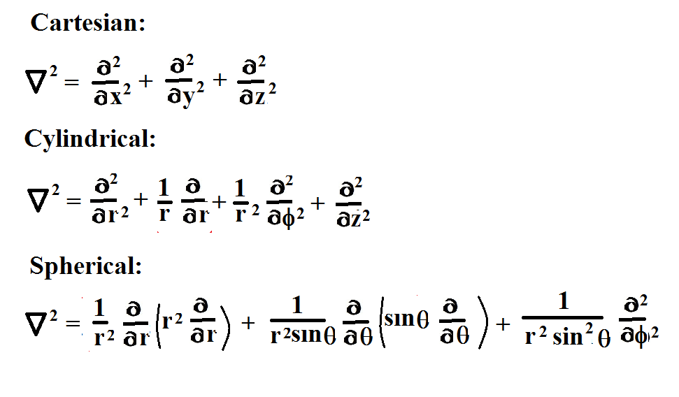
These diagrams shall serve as references while we derive their Laplace operators. Here's what they look like:

The Cartesian Laplacian looks pretty straight forward. There's three independent variables, x, y, and z. The operator has three terms as one would expect, but check out the cylindrical operator--it has four terms and three variables. What's up with that? If you examine both the cylindrical and spherical operators, you notice terms that have factors in front of the partial derivative operators. Where do they come from and why are they necessary? To answer such questions, it pays to derive these operators from scratch.

In this post, we derive all three Laplace operators, so a side-by-side comparison can be made which further illuminates the logic behind the derivation procedure. Let's begin by expressing an arbitrary vector S in terms of each coordinate system:

The next step is to extract the unit vectors. This is done by taking partial derivatives of S with respect to each variable. For the Cartesian version, this is totally straight forward:

No normalization is required because dot products of the unit vectors give you 1's and 0's as expected:

Now, here's what we get when we take partial derivatives of the cylindrical version of S:

The unit vectors we get aren't really unit vectors. When we do dot products, we don't necessarily get 1's and 0's. Normalization is required:

Notice that one of the partial-derivative operators requires a normalization factor of 1/r. Spherical unit vectors also require normalization:

Here, two spherical partial-derivative operators require a normalization factor: 1/r and 1/rsin(theta) respectively. Now that we know the normalization factors, we can construct the gradients:

Notice how the unit vectors are placed in front of the partial-derivative operators. A common mistake is to place the unit vectors after the operators like this:

This is technically wrong or should be, since the operators are acting on the unit vectors! Here's what happens:

So we keep the unit vectors in front. This prevents errors and frustration as we perform the next step which is to square the gradients to get the Laplace operators. Let's do the easiest one first, the Cartesian gradient. We multiply each term by every other term. Doing so allows us to construct this matrix:

Here's a couple of examples of the multiplication procedure. Note that the product rule of derivatives is employed and the partial-derivative operators do in fact operate on the unit vectors, but only where it's appropriate:

The final answer is ...(drum roll) ...

Now let's square the cylindrical gradient using a similar procedure:

Looking at each term it is obvious, that once again, there is a partial-derivative operator acting on a unit vector. We can make a list of each operation we will encounter, then use the list data to make the necessary substitutions during the multiplication process.

And here's the math for the cylindrical Laplacian:

Here's the final answer:

Finally, we tackle the spherical Laplacian:

The second matrix above indicates which terms give us zero when we do the math. Below we focus on the terms that yield a value other than zero:

We gather up the terms:

Too many terms! Here's what we can do. Let's take the first couple of terms and factor out 1/r^2. Then apply the derivative product rule in reverse:

Next, take the following terms and factor out 1/{(r^2)sin(theta)}. Once again, apply the product rule in reverse:

After making substitutions, the final answer is ... (fireworks) ...