How to Have Unlimited Orthogonal Space and Time Dimensions within 4D Spacetime

ABSTRACT:

By means of a thought experiment and a mathematical proof, it can be shown that unlimited space and time dimensions are possible, and, that only three space dimensions are mutually perpendicular.

Imagine you are throwing a party. You have invited n number of guests. You want to know the following: the starting location and time of each guest and the time each guest arrives at your party. You know the location of the party and you know what time the guests are supposed to arrive. All of this information consists of 2n+1 bits of time and n+1 bits of location. Assuming each location has coordinates x, y and z, the total bits of space information is 3n + 3.

Each bit of information is statistically independent, i.e., orthogonal to all the rest. We can think of any two bits as having a 90 degree separation. In the case of coordinates x, y, and z, such separation can be easily drawn on graph paper. In all other cases, such separation may be purely abstract and unimaginable. In any case, we can argue that 3n+3 space dimensions and 2n+1 time dimensions are necessary. To have all the information you want, you need 5n+4 dimensions. If n = 100 guests, you only need 504 spacetime dimensions!

It's fairly obvious that the above thought experiment only involves three space dimensions that are mutually perpendicular. But is this universally true? Is there, say, a mathematical proof? The following equation suggests there's no upper limit to how many space dimensions you can have:

It seems like the only constraint re: the number of space dimensions is an empirical one. Let's see if we can find a mathematical one. Let's begin with the following premises:

1. w, x, y and z are unit vectors.

2. w is an arbitrary extra space dimension. What is true for w is true for any extra space dimension.

3. A unit vector is consistent with 1D space and points in only one direction.

4. if two unit vectors (x, y) are perpendicular, they define a plane that is consistent with 2D space. Thus plane xy is not perpendicular to plane xy.

Following these premises we have:

At steps 2 through 4 we assume that all four unit vectors are mutually perpendicular. At 5 we assume w is perpendicular to plane xy. At 6 we assume z is also perpendicular to plane xy. At 7 we conclude that either w is parallel to z or if w is perpendicular to z, then plane xy must be perpendicular to plane xy--which violates premise 4. So w is not an extra dimension. According to premise 2, what is true for w is true for any alleged extra space dimension. Thus, we can further conclude there are only three space dimensions that are mutually perpendicular. If such a conclusion is valid, we should be able to falsify the following 7D cross product table:

From this table we can gather that the unit vector e1 is the solution to three cross-products involving 6 dimensions (see equation 8 below). Premise 3 stipulates that a unit vector only points in one direction. It is also obvious that e2e3, e4e5, e6e7 make three planes persuant to premise 4. Vector e1 can't point in just one direction if it is normal to all three planes, unless all three planes are subsets of the same plane. The inevitable conclusion is not all of these dimensions are mutually perpendicular.

Now, let's take a look at the so-called extra dimensions 4 through 7. At each of the equations 9 through 12 below, the unit vectors circled in red contribute to planes with normal vectors pointing in different directions. Thus they can't all have the same normal vector or cross-product solution.

Therefore, it is safe to say that dimensions 4 through 7 do not behave like mutually perpendicular dimensions.

Circling back to our hypercube at equation 1, we can conclude that there is no upper limit to how many dimensions the cube can have, but only three are mutually perpendicular. The rest may or may not be orthogonal in the sense that they are statistically independent.

References:

1. Seven-dimensional Cross Product. Wikipedia

2. Octonian. Wikipedia

Resolving the Liar's Paradox: "This Statement is False"

"I am a liar," is the original liar's paradoxical statement, but we're going to focus on one of its variations: "This statement is false." If true, then it is false. If false, it must be true. To resolve this paradox, we begin with the following premises:

1. If a statement is true or false, it is one or the other and not both, and, we can determine whether it is true or false.

2. If a statement is true and false, it is a challenge to give it a truth value.

Now let's define some statements: Statement A = "This statement has five words." Statements B and C = "This statement is false." Statement D = "This statement has four words."

Given the foregoing premises, we can determine the truth value of each statement using an AND-gate truth table and by following these steps:

1. Read the statement and determine if it is true or false. If this can't be done, assume it is true (or false if you prefer). Mark the left side of the truth table T for true or F for false.

2. Then ask, "If I assert the statement is true (false), does it become false (true)? If not, repeat your previous mark. If so, add the opposite mark.

If these steps are followed, the truth table for statements A, B, C, D should look like this:

For the true statement A, there is no contradiction or paradox so the two marks are TT. Statement B equals statement C. At B we start out assuming the statement is true, and, at C we begin assuming it is false. That leads to scores TF and FT, respectively. Statement D is determined to be false and remains false, so we have FF. At the far right column are the final truth values. The true statement is true; the false statement is false, and, the paradoxical statement is false. This last result is consistent with the law of non-contradiction. Statements that are contradictory or lead to a contradiction are not credible and should be considered false, notwithstanding any claim to the contrary.

References:

1. Mano, M. Morris and Charles R. Kime. Logic and Computer Design Fundamentals, Third Edition. Prentice-Hall, 2004. p. 73.

2. Epimenides paradox has "All Cretans are liars." Titus 1:12

3. Jan E.M. Houben (1995). "Bhartrhari's solution to the Liar and some other paradoxes". Journal of Indian Philosophy. 23 (4): 381–401.

4. Hájek, P.; Paris, J.; Shepherdson, J. (Mar 2000). "The Liar Paradox and Fuzzy Logic". The Journal of Symbolic Logic. 61 (1): 339–346.

5. Mills, Eugene (1998). "A simple solution to the Liar". Philosophical Studies. 89 (2/3): 197–212.

Debunking Extra Space Dimensions and Minimum Distance

ABSTRACT:

By means of two thought experiments and some mathematics this paper shows that extra space dimensions are untenable. This paper also shows that the minimum distance is many orders of magnitude shorter than the Planck length.

Imagine a 2D universe on an x-y plane (see diagram below). Imagine a normal vector intersecting this plane at point p. 2D-guy inhabits this universe. He can't see the vector that intersects point p. He can only detect point p, so he has no reason to believe the normal vector exists. Now, to avoid point p, he goes around it (see red arrows).

He knows it's possible to draw an imaginary line through point p that can serve as an axis. He also notices when he goes around point p he's not encircling the x-axis or the y-axis--the two dimensions of his space. Thus, he infers that the imaginary axis he's going around does not belong to his 2D universe. He realizes he has discovered a new dimension!

Now, what happens if we apply 2D-guy's process to 3D space? Will we discover a fourth dimension? Let's try it. First we must scale everything up one dimension: The universe becomes 3D; the normal vector becomes a normal plane; Point p becomes line L. Let's assume there's a fourth dimension w, and let's define the normal plane as wx. Plane wx intersects our universe at line L which runs along the x-axis. We should not be able to detect the w-axis nor the bulk of the wx plane. We illustrate this with broken lines at the diagram below:

To avoid line L, we circle around it (see red circular path). We know we can draw an imaginary plane through line L. We know that x is one dimension of the plane. We know the axis we are circling (to avoid line L) is the plane's other dimension. We note we are not going around the x-axis nor the z-axis. That leaves the w-axis, but notice that the w-axis is indistinguishable from the y-axis. Therefore, our assumption that w is a new dimension and is undectable beyond line L is false. Unlike 2D-guy, we have not discovered a new dimension. However, we learned from 2D-guy that if a new dimension exists, it should be possible to do a rotation around an axis that does not exist in our universe. Until someone demonstrates such a rotation, we can conclude, for now, that the highest dimension of space is 3D.

But what if there are extra dimensions that are very small and curled up? If that's the case we should be able to enter alternate universes and those from alternate universes should be able to enter ours. Let me demonstrate what I mean. Imagine a line and pretend it is 3D space. Extending from it is a small extra curled-up dimension:

Let's introduce an arbitrary red object that is way too big to enter the tiny curled-up dimension:

Because the red object is too big to fit, it is assumed there is no way for the big red object to enter or detect the existence of the curled-up dimension. But didn't Euclid say something about a line existing between any two points? (In this case the line would be 3D.)

There's no reason why the big red object can't follow the path of this new line (3D space)and wind up in an alternate universe adjacent to ours:

As you can see, the big red object still can't enter the small, curled-up dimension, but the curled dimension facilitates access to alternate universes. The fact that big objects don't disappear from our universe and don't seemingly emerge from nowhere is strong evidence that microscopic curled-up dimensions don't exist. But wait! Quantum particles pop into existence and vanish all the time. It is hypothetically believed they enter a curled-up dimension (vanish), then leave that dimension and re-enter our universe. However, there's an alternate hypothesis: particles are really particle-waves. Waves experience constructive and destructive interference. When there's an excitation of a field, a particle pops into existence. That excitation could be or is equivalent to constructive interference. When there's destructive interference, energy vanishes--leaving the impression that the particle has disappeared.

The foregoing arguments seem to kill any notion that there are more than three space dimensions, but what about 4D spacetime? Or, what about the 6D object that can be found in Las Vegas? Let's address the 6D object first.

The 6D object I'm referring to is the die. The die has six orthogonal sides. Each side is statistically independent. We can change the value of a side without impacting the value of the other sides. If we change, say, the one to a seven, the other sides will still be two, three, four, five, and six. The most important point we can take away from the die is it is possible to have more than three orthogonal dimensions within 3D space! The die is a 6D object but it is also a 3D cube.

Spacetime, on the other hand, involves three dimensions of space and one dimension of time. If time is multiplied by a velocity, it has units of distance and is treated as a fourth space dimension. But is it really? Let's see what the math has to say:

Equation 1 represents a photon propagating through dimensions x, y, and z over a period of time t. It covers a distance of ct or r. For the sake of keeping the math simple, at equation 2 we rotate the path r so it is along the x-axis. Equation 3 reveals that space and time are not statistically independent, i.e., orthogonal to each other. The the value of time t depends on how far the photon propagates along x, and the value of x depends on how much time t lapses. This is the consequence of converting t into distance units by multiplying it by velocity c. So ct is not a true space dimension that is orthogonal to x. However, time t without c is a very useful statistically-independent parameter. For example, coordinates x, y, z tell you where to be for your dentist appointment and time t tells you when. A change in location does not have to change the time of the appointment, nor does a change in time have to change the location. So what can be done to make ct orthogonal to x? How about multiplying ct and x by factors of g? (See equation 6.) A change in x still causes a change in t, but g-sub-tt can be adjusted so the term stays constant. By the same token, the other term stays constant if g-sub-xx is adjusted when a change in t changes x.

So can we now credibly argue that (g-sub-tt)ct is a genuine fourth space dimension? Well, no 3D space dimension (x,y,z) has to be a function of (depend on) the others. We can, for example, eliminate y and z and still have x. But we can't eliminate a photon's path (x, y and/or z) and still have ct--the distance along a non-existent path. And, if there's no ct, then there's no (g-sub-tt)ct. Therefore, (g-sub-tt)ct is a pseudo-dimension at best.

So far, it seems we've only debunked a fourth dimension of space. What about dimensions five through infinity? Well, how we label a dimension is arbitrary. Any extra dimension can be labeled the fourth dimension. Thus, all arguments we have made against dimension four apply to any extra space dimension.

Now let's turn our attention to the concept of the shortest distance. The popular choice is the Planck length. In fact some theorists quantize space with Planck-size cubes or Planck-size tetrahedrons or Planck-size strings:

In the above diagram, the cube and tetrahedron have sides that are each one Planck length. However, the red diagonal lines reveal shorter lengths all the way down to a single point. These shorter lengths are absolutely necessary to create the shapes desired. Without a zero-length point, for example, there can be no corners for cubes and tetrahedrons. Additionally, there can be no strings in any string theory, since a string is a 1D object. A 1D object implies a zero cross-section or single point. A minimum-distance-greater-than-zero requirement would be a nightmare for M-theorists, since all D-branes would have to be 10 dimensions (including strings!). To have less than 10 dimensions requires zero distance for one or more dimensions. So it can be argued that the minimum distance is really zero, at least on paper. What about the physical world?

Equation 7 tells us that the shortest wavelength is determined by the highest energy. When the universe was a singularity, how short was the singularity's wavelength? If we only account for the energy in the known universe, that wavelength would be approximately a Planck length of a Plank length of a Planck length! Not exactly zero, but far less than a Planck length. Add energy beyond our known universe, and the distance is even shorter.

From a philosophical standpoint, the very concept of length implies a 1D object in the same manner the concept of area implies a 2D object. To measure length requires that we ignore all but one dimension, i.e., we set all but one dimension to zero. So zero distance is necessary, at least in the mind's eye. Since the mind's eye lives in this universe, we can infer that the minimum distance in this universe is zero.

In conclusion, any extra space dimension would allow rotations around an imaginary axis that is not part of 3D space. It would also allow any object access to an alternate universe. The shortest distance is many orders of magnitude shorter than the Planck length, and the Planck length may only be a lower limit of what we can successfully measure.

References:

1. Greene, Brian. 2003. The Elegant Universe. W. W. Norton

2. Irwin, Klee. 04/23/2017. The Tetrahedron. Quantum Gravity Research.

3. Sutter, Paul. 02/23/2022. Loop Quantum Gravity: Does Space-time Come in Tiny Chunks? Space.com

Curing Divergences without Supersymmetry and Renormalization

Abstract:

Supersymmetry or ad hoc methods such as renormalization are often used to tame infinities that result from divergent functions in quantum physics. Although SUSY particles have yet to be discovered and may be too massive to fulfill their purpose, and, renormalization seems to lack mathematical rigor. Here we offer an alternative method that employs the least-action and Heisenberg uncertainty principles.

Imagine a Lagrangian with divergent terms. One strategy is to renormalize it. Simply discard the divergent terms, especially if they are infinite. However, Paul Dirac had this to say about such methods: "I must say that I am very dissatisfied with the situation because this so-called 'good theory' does involve neglecting infinities which appear in its equations, ignoring them in an arbitrary way. This is just not sensible mathematics. Sensible mathematics involves disregarding a quantity when it is small – not neglecting it just because it is infinitely great and you do not want it!"

Another strategy is to add superpartners that each have the same mass as their respective standard-model counterparts but make an opposite contribution to the Lagrangian. As a result, the divergence vanishes. Albeit, there is a slight problem: the symmetry of Super-symmetry is broken--the superpartners are believed to be more massive than their standard-model partners. This deflates the balloon of vanishing divergences. To make matters worse, there is a complete and total lack of empirical evidence supporting these superpartners.

If renormalization seems like bad math and SUSY particles are nowhere to be found, what other options are there? How about the least-action and Heisenberg uncertainty principles? Let's first examine the least-action principle:

A particle typically takes the shortest path possible between two points. For that to happen, delta-s, at equation 1, cannot be a large, divergent quantity. It should be zero units of action or time multiplied by energy. However, the following is true:

Line 3 shows that time multiplied by energy is greater than or equal to h-bar. To get delta-s to equal zero requires steps 4 through 6:

At 7 we set up another substitution. The final equations are 8 and 9 below:

Equations 8 and 9 show why there's a least action principle and why energy is generally conserved. Suppose we have a conserved energy L. The divergent energy, delta-E, can be interpreted as energy borrowed from the vacuum. Because it's borrowed, it must vanish within time delta-t. The larger this energy, the shorter its lifespan. As a result, the energy L that you start with is the energy you end up with. It is conserved. Also, the action is the least action.

At equation 10 we have a Lagrangian where there is no borrowed energy. Because no energy is borrowed, time delta-t is infinite. In other words, this scenario can last indefinitely and create the impression that energy is always conserved.

At equation 11 we have the opposite extreme: a Lagrangian that diverges to infinity. The good news is delta-t is zero, which shows that infinite borrowed energy does not exist. We can also infer that large borrowed energies exist for too short of a time to be meaningfully observed and measured, so the energy we do observe and measure is small by comparison. Thus, renormalization works despite its ad hoc nature because nature wipes out divergences by means of the uncertainty principle and least action. The only time it is appropriate to keep the divergent terms is when divergent energy is added to the system and not borrowed from nothing.

Now, let's suppose L is a Lagrangian for vacuum energy (see equation 12). A Higgs boson (m-sub-H) pops into existence and has a lifespan of t-sub-H. A too-large Higgs mass would have a lifespan too short to provide a meaningful opportunity to observe it, so the mass we are most likely to observe is a smaller mass.

More examples: Equation 13 below takes into account multiple particles. Equation 14 takes into account a Lagrangian or function with multiple terms and parameters.

Since delta-s must be zero to minimize the action, then delta-s along D dimensions must also be zero. Further, both delta-s and s have units of momentum multiplied by position. If we integrate over position and/or momentum space, the following must be true:

The uncertainty of knowing a particle's position is cancelled by knowing its momentum and vice versa. As a result, the particle's action is minimized along with its position path and momentum.

In conclusion, divergences are tamed if the least-action and uncertainty principles are applied. SUSY particles are not needed and ad hoc methods such as renormalization can be set aside.

References:

1. Lincoln, Don. 2013-05-21. What is Supersymmetry? Fermilab.

2. Martin, Stephen P. 1997. A Supersymmetry Primer. Perspectives on Supersymmetry. Advanced Series on Directions in High Energy Physics. Vol. 18.

3. Susskind, Leonard. 2012. Supersymmetry and Grand Unification Lectures. Stanford University

4. McMahon, David. 2008. Quantum Field Theory Demystified. McGraw Hill

5. Baez, John. 11/14/2006. Renormalizability. math.ucr.edu

6. Renormalization. Wikipedia

Giving Neutrinos Mass by Adjusting the Higgs and Electroweak Mathematics

ABSTRACT:

This paper shows a new mathematical algorithm that allows weak-force bosons to have mass and leaves photons massless while giving mass to neutrinos and other leptons.

The right side of equation 1 below is the Higgs vector used to ensure that photons don't have mass and that the weak-force gauge bosons have mass. This same vector also ensures that leptons will have mass except for neutrinos.

Neutrinos, however, are not massless. This fact indicates that the electroweak theory is not complete. To fix the theory we need something like the vector on the right side of equation 2:

This new vector compensates for whatever contributes to neutrino mass. If we use this new vector when determining masses for leptons, and, use the old vector for determining masses for gauge bosons, we end up with the status quo and the extra bonus of slightly massive left-handed neutrinos.

To theoretically justify this new vector we'll examine how the old vector was derived from a Lagrange potential. We will make a minor adjustment to this Lagrange potential without changing its value and its gauge translation invariance. The minor adjustment will allow a derivation of the new vector as well as the old. Here is the Lagrange potential in its original form:

Equations 3 through 6 demonstrate gauge translation invariance and lead to equation 7. Next, we take the derivative with respect to phi to acquire the minimum potentials:

At 11 and 12 above we have the minimum potentials we find in the Higgs vector at equation 1. To derive the new vector at equation 2 we do the following:

Two new terms are added to the potential that cancel each other, so the potential is the same. Once again gauge translation invariance is demonstrated. After all is said and done, we have two useful equations: 18 and 19. If we substitute the zero value at 18 into 19 we have the original Lagrange potential. Once again, we can take the derivative and derive the original Higgs vector. Or, we can take the derivative of equation 19 without the substitution:

At 23 we end up with two non-zero solutions. If phi is small, we have the first approximate solution. If phi is larger we have the second approximate solution. This is consistent with, say, an electron being more massive than its family neutrino. We now have what we need to create the new vector (see equation 2).

The next step is to show how this new vector is applied. When the mathematics is normally done, all terms containing h(x) are discarded at the end, but the solutions don't change if we discard h(x) early or leave it out of the vector. Doing so greatly streamlines the math. Thus the new vector becomes

There are three families of leptons. Since the same mathematics applies to all three, let's just focus on the electron family. The normal interaction Lagrangian for the electron family is

The problem with this Lagrangian is it assumes the left-handed neutrino has no mass, so we need to adjust the Yukawa coupling Ge to G.

Since the right-handed electron doesn't have a corresponding right-handed neutrino, the Greek letter nu with an R subscript has a zero limit at equation 30. After performing the matrix operations we get

Now let's set up some substitutions and define the modified Yukawa coupling G to include neutrino and electron masses:

The final results are below. At 37 we have the left-handed neutrino's mass. At 38 we have the electron's mass (notice how the adjusted Yukawa coupling coupled with the new groundstate equals the standard Yukawa coupling coupled with the original groundstate. Both terms equal the electron's mass.)

The forgoing exercise can be repeated for the other two families of leptons. To account for different masses, simply use different Yukawa couplings.

In conclusion, to give neutrinos mass requires a new Lagrange potential that can yield two field vectors: one for gauge bosons and one for leptons. Also, Yukawa couplings for massive neutrinos need to be added. When these requirements are met, the final solution shows that left-handed neutrinos do indeed have mass.

Quantizing Gravity without the Graviton

Abstract:

This paper shows the connection between "dark energy" and gravity, the equivalence between matter and space, and how gravity works without the graviton or gravitational waves. It also suggests an alternate way to quantize gravity using smaller units--of mass, space and time--than the Planck units.

The same force acting on different masses will cause each mass to move at a different rate: F = ma, where m is mass and a is acceleration. However, the same "gravitational force" causes different masses to fall at the same rate. How can this be? Einstein proposed that when a body appears to be falling to earth, it is really at rest, and the earth is accelerating towards the body at a given rate. Thus the body's mass is irrelevant.

Below is a diagram of Alice who is surrounded by four bodies, including Bob. Bob and the others appear to be either moving away from Alice or towards her, depending on how you follow the arrows. But if we go from left to right, we can think of Alice as the one who is moving away from the surrounding bodies. If we go from right to left, we can think of Alice as the one who is moving towards the surrounding bodies. As a consequence, the surrounding bodies can have any mass and the rate at which Alice and the surrounding bodies diverge or converge will be the same.

Equations 1 and 2 below were derived from Einstein's field equations. Equation 3 was derived from a Friedmann equation where k is set to zero due to spacetime being flat at a large scale where the mass density (rho) is a small number and so is the curvature which is represented by the cosmological constant.

At 4 and 5 we set up a couple of substitutions to be made at 7 and 8 below. Equation 6 shows how mass and space are equivalent. Divide any mass by the vacuum-mass density to get the equivalent volume. Equation 7 shows the universe must expand faster than light as the radius r tends to infinity; otherwise, light speed in a vacuum is not conserved! If both sides of the equation are multiplied by the universe's mass, then the universe's energy is conserved no matter how big or small the universe becomes.

Also, the vacuum-mass density rho correlates with outward pressure, and that pressure is not diminished by an increase in distance r, so the outward pressure continues and so does the universe's expansion. At equation 8 we see that gravity looks similar to equation 7. As the speed of gravity increases, it is offset by the increase in spacetime curvature. As a result, the constant c and energy are conserved.

Equation 9 below shows that gravitational waves are caused by gravity and angular frequency, so they cannot be the cause of gravity. In fact, if angular frequency is zero, there is still gravity but no gravitational waves.

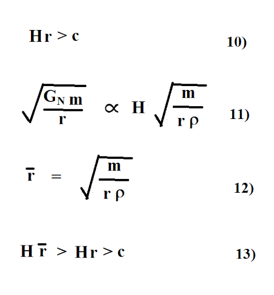
Now, let's imagine Alice and Bob are so far apart that Bob is moving away from Alice faster than light (see 10 below). Alice starts out with very little mass, but decides to go off her diet. As a result, she gains an enormous amount of mass. So much so that she becomes a black hole (see equation 11). The distance between her and Bob is the same but it is now less than Alice's Scharzschild radius. So are Alice and Bob still diverging or are they now converging?

We know that no signal, limited to light speed, ever reached Bob. This includes gravitons, gravitational waves, light, etc. At 12, Alice's mass is converted to it's equivalent space. Finally, the inequality at 13 shows that Bob is still moving faster than light if Alice is at rest, but Alice is no longer at rest--she's moving faster than Bob towards Bob. Thus Alice and Bob are converging as if a "gravitational force" is present.

Take a proton and electron. Equation 14 below shows acceleration depends on both their respective charges, their masses and distance r. Clearly there is an information exchange between them. At equation 15 it's a different story: acceleration only depends on the mass of the proton and distance r. It is clear the two masses don't exchange information. It's as if the proton simply accelerates towards the electron.

Now, let's consider Alice, Bob and Carl below. How fast Alice accelerates depends on the distance of the targets, the targets being Bob and Carl. Surely Alice needs to know the distance of each target so she can adjust her rate of acceleration accordingly?

Consider the diagram below. The numbers in each section add up to the total volume of the 3X3X3 cube. At 17 the volume of each cube is divided by its square. If we multiply each term by the square of Hubble's parameter it becomes apparent that Alice is accelerating less than Bob and Bob is accelerating less than Carl. These three are diverging as if they are in an expanding universe.

Now, let's add mass to the red section. Let's convert it to its equivalent volume which is 100 units. That brings the total to 101 units. Notice that the state of Bob's section (blue) and the state of Carl's section (green) do not change. Each have their previous volume. Also notice that the square areas do not change. This implies no information exchange between Alice, Bob and Carl. But now Alice is accelerating more than Bob and Bob is accelerating more than Carl. The three are converging is if they are in a gravitational field.

The rate of acceleration depends on distance but, as demonstrated above, this does not imply an information exchange between the parties. To drive this point home, imagine we divide up our universe into volume cells, each cell expands at a given rate independently of every other cell. More cells cause a greater rate of expansion, but each cell has no clue how many cells an observer is looking at or what the other cells are doing. The cells exchange no information. Thus the rate of expansion is really up to the observer. Now, suppose you add more volume (cells) to the system without increasing the space. This was done when mass was added to Alice's section (red). Mass's equivalent volume doesn't change the distances between Alice, Bob, and Carl. The result is what we call gravitational acceleration (see equation 20 below). Again, each cell need not know the state of the others. The rate of acceleration depends on the distance the observer chooses to consider.

Now let's turn to quantizing gravity. The popular choice is, of course, the graviton, but the graviton causes a major setback. If we assume the graviton is a real thing, surely we can come up with a reasonable estimate of how many gravitons are in the universe. For example, we could figure the total gravitational energy of the universe and divide that by the average energy of the graviton. At 21 below we plug in the entire mass of the universe to get the gravitational energy, but we don't get units of energy. Instead, we get velocity squared. One could argue that there is no gravitational energy, so there are no gravitons. Equation 22 is an attempt to counter this argument. It uses two masses which give an energy term, but how much gravitational energy there is depends on how much of the universe's total mass we assign to m and m'. Also, whatever gravitational-energy total we arrive at will be exceeded by a single black hole singularity and a single particle that have virtually zero distance between them.

At equation 23 we switch to a smaller scale. We assume the gravitational energy produced by an electron and proton is nEg, where Eg is the energy of one graviton and n is the number of gravitons. Therefore two electron-proton pairs produce 2nEg or 2n gravitons? Not so fast. Since gravitons have energy, they also produce gravitons. At 24 they produce up to an infinite number of gravitons if the distance r limit is zero! So how many gravitons are in the universe? It depends on how you crunch the numbers.

By contrast, it is much easier to estimate how many photons are in the universe, since photons don't produce photons. Electromagnetic energy is a function of charge and not energy or mass. So as long as photons don't have charge, they don't infinitely reproduce themselves. We can take the total luminous energy of the universe and divide it by a photon's average energy to get a reasonable estimate of how many photons there are.

For the above reasons, the graviton is untenable. So then how should we quantize gravity? Gravity is a function of mass (defined as energy divided by light speed squared), space and time. Thus it would make sense to quantize these fundamental dimensions. We could ask, what is the shortest length or time, and, what is the smallest mass? The popular response is, the Planck length, the Planck time and the Planck mass, respectively. But are these really the smallest units? The Planck mass clearly is not the smallest mass. An electron mass is smaller. Also, the Scharzschild radius of an electron is much shorter than a Planck length. The time it takes for a photon to travel the shorter distance is less than the Planck time. So what are the smallest units? Here are the smallest units I have found so far. I call them the Hubble units:

We could take the Hubble length, for example, and quantize equation 13 as follows:

At equation 29 the first term has alpha Hubble lengths; the second term has beta Hubble lengths. The smallest rate of expansion is Hubble's parameter times one Hubble's length. Now, one probable objection to this scheme is space is chaotic and stochastic on the quantum scale, so how can we have such nice, neat units? The Hubble length, for example, could be an expectation value (average) of all the chaotic activity that may make up space. We can think of the Hubble units as perhaps the smallest average units that can be derived from fundamental constants and Hubble's parameter.

In conclusion, unlike the other fundamental interactions, gravity does not appear to have any means for bodies to communicate with each other, nor is communication necessary. Thus the graviton is unnecessary. Further, the graviton fails to conserve energy like its electromagnetic counterpart the photon. A better way to quantize gravity is to quantize space, time and/or mass.

Acknowledgments:

Amber Strunk. Education and Outreach Lead. LIGO Hanford Observatory.

Peter Laursen, Astrophysicist and science communicator at the Cosmic Dawn Center, University of Copenhagen.

References:

1. Parikh, Wilczek, Zahariade. 2020. The Noise of Gravitons. arxiv.org.

2. Feynman, R.P. 07/03/1963. Quantum Theory of Gravitation. Acta Physica Polonica. Vol. XXIV.

3. Graviton. Wikipedia.

4. Carlip, S. 12/1999. Aberration and the Speed of Gravity. arxiv.org.

5. Van Raamsdonk, M. 05/17/2010. Building up spacetime with quantum entanglement. arxiv.org.

6. Hanson, R.; Twitchen, D. J.; Markham, M.; Schouten, R. N.; Tiggelman, M. J.; Taminiau, T. H.; Blok, M. S.; Dam, S. B. van; Bernien, H. (2014-08-01). Unconditional quantum teleportation between distant solid-state quantum bits. Science. 345 (6196): 532–535.

7. Gravitational Wave. Wikipedia.

8. de Rham, C., Tolley, A.J. 03/17/2020. Speed of Gravity. arxiv.org.

9. Carroll, S.M. 12/1997. Lecture Notes on General Relativity. Enrico Fermi Institute.

10. Marsh G.E., Nissim-Sabat. 3/18/1999. Comment on an article by Van Flandern on the speed of gravity. Physics Letters A Vol. 262, pp. 257-260 (1999)

11. Suede M. 11/29/2012. The Speed of Gravity: Why Einstein Was Wrong and Newton Was Right. Blog commentary re: Tom Van Flandern.

12. Cornish N., Blas D., and Nardini, G. 10/18/2017. Bounding the Speed of Gravity with Gravitational Wave Observations. Phys. Rev. Lett. 119, 161102

13. Van Flandern, T. 1999. The Speed of Gravity What the Experiments Say. Meta Research University of Maryland Physics Army Research Lab.

14. Nix, E. 08/22/2018. Who Determined the Speed of Light. History.com.

15. Speed of Gravity. Wikipedia.

16. Tests of General Relativity. Wikipedia.

17. Decross, M. et al. Gravitational Waves. Brilliant.com.

18. Lawden, D.F. 1982. Introduction to Tensor Calculus, Relativity and Cosmology. Dover Publications, Inc.

19. Stefanovich, E. V. 09/16/2018. A relativistic quantum theory of gravity. arxiv.org.

20. Light-time correction. Wikipedia.

21. Liénard–Wiechert potential Wikipedia.

22. Kopeikin, S. M. Fomalont, E. B. 03/27/2006. Aberration and the Fundamental Speed of Gravity in the Jovian Deflection Experiment. arxiv.org.

23. Faber, J. A. 11/24/2018. The Speed of Gravity Has Not Been Measured From Time Delays. arxiv.org.

24. Yin Zhu. 08/18/2011. Measurement of the Speed of Gravity. arxiv.org.

25. Perihelion of Mercury’s Orbit. macmillanlearning.com.

26. Belenchia A, Wald, R.M., Giacomini, F., Castro-Ruiz, E., Brukner, C., Aspelmeyer, M., 03/22/2019. Information Content of the Gravitational Field of a Quantum Superposition. Gravity Research Foundation.