Why Are There Opposite Charges?

Why are there opposite charges? According to at least one string theory, a charge is caused by a string wound around a cylinder that contains a hidden dimension through its cross-section. If the string is wound in one direction, the charge is positive. If it is wound in the opposite direction, the charge is negative. Below is a diagram of the model:

The problem with this model is you have a hidden dimension and a string. This creates a greater burden of proof for the physicist. The physicist must now discover strings and extra dimensions. Good luck! Plus it looks man-made and not natural. Finally, it is not intuitive or obvious why a plus charge is attracted to a minus charge or why same charges repel.

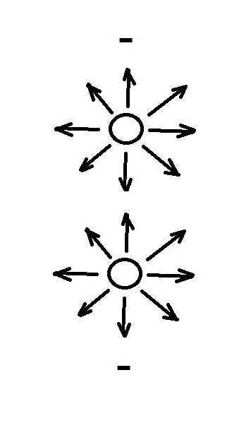
Question: why is the string and extra dimension necessary? Below is a model where the extra dimension and string are removed. It is simply a point with arrows that represent field lines. When the arrows go in, the charge is positive; when the arrows go out, the charge is negative.

The diagram below shows two negative particles. Notice how the arrows (field lines) between them look like they are pushing against each other--like two rivers flowing against each other. This is consistent with the fact that they repel each other.

In the next diagram we have two positive particles. Notice how the field lines (arrows) between them look like they are moving away from each other. This is consistent with them repelling each other.

The final diagram below shows a positive particle interacting with a negative particle. Notice how the arrows flow in the same direction. They don't push against each other, nor do they move away from each other. This is consistent with attraction.

As you can see it is possible to build a more intuitive model that demonstrates opposite charges without increasing our burden of proof, i.e., without adding extra dimensions and strings.

Why Does Squaring a Wave Amplitude Yield a Probability?

Perhaps you heard the story (that's code for unsubstantiated rumor) where Paul Dirac, a legend in the field of quantum physics, woke up one morning, put on his trousers, put on his shirt, put on his socks and shoes. He then stepped into the shower, forgetting he had already dressed. His mind was elsewhere, but the brisk chill of cascading water drenching his clothes brought him back. "That's it!" he said. "Square the amplitude and you get the probability!"

He was, of course, referring to the fact that you can take the inner product of an eigenvector (or ket) with its complex conjugate (bra) and get a probability of a particle's position, momentum, or whatever. It's a pretty cool trick and it works. The question is why? Why does squaring a wave amplitude yield a probability? Below is a mathematical equation that I thought up while I was taking a shower (with my clothes on):

In the numerator you may recognize Euler's identity. Basically, the numerator is the sum of all possible wave amplitudes. The denominator is a normalization factor: it ensures that when you calculate the inner product of the equation's right-side expression with its complex conjugate you get one. One is a good number to get, since it is the sum of all probabilities. Most importantly, the equation shows the connection between wave amplitudes and probabilities.

Below is a visual aid that I hope will clarify the connection. It is a well-known fact in the subject of trigonometry that sine squared plus cosine squared always equals one. This fact can be used to model not only waves, but probabilities as well, since the sum of all probabilities also equals one. However, to reach a total of one, one must divide the wave amplitude by X1 in the case below where n is equal to one, i.e., where there is only the sum of one Euler's identity multiplied by a coefficient X1.

The lower part of the visual aid shows the inner product between the bra and ket vectors.

As you can see in the diagram below, the sum of squared wave amplitudes equals one, and probabilities P(A), P(B) add up to one.

This system works well if you have only two probabilities: cosine squared can represent one probability and sine squared can represent the other, but what if there are three or more probabilities? Well, that's why I put together the equation we started with. Let's say there are three probabilities, and they must add up to one. In such a case we need to raise n to 2:

There are now three wave amplitudes. When you square them, add them, and divide by the normalization factor (x1^2 + x2^2), you get one. You also get one when you calculate the inner product of the bra-ket vectors:

And, of course, the probabilities also add up to one:

Unifying the Schwarzschild Metric and Quantum Physics

Is it possible to unify quantum physics with Schwarzschild's metric for black holes? Absolutely! All we need to do is adapt my relativity wave function to the task. For more information on the relativity wave function, click here.

Here is an example of the function:

It consists of Euler's identity and more than one k variable (bar-k's to be exact). Time is t; light speed is c, and i is an imaginary number. The variable rs below is the Schwarzschild radius; a and b are terms from the Schwarzschild metric, and r is the radius. Our first step is to transform the bar-k's. For example, bar-k(1) becomes ak(1).

Next, we trade Cartesian coordinates for spherical coordinates. Here is what we get:

We can now express the Schwarzschild metric in quantum mechanical terms:

When the partial derivatives above are solved, we get the standard Schwarzschild metric below:

Looks rather messy. Let's put the variables into a more manageable form:

When the function is used in Schrodinger's time-dependent equation (complete with potential energy V, the Laplacian, and Planck's constant, h-bar), here is what results:

Time to substitute the real values of a and b--but Huston we have a problem! Notice when r is equal to rs, we have zero on the equation's left side and infinity on the right side. The equation works fine as long as the particle is far far away from the black hole's horizon, i.e., when r is a big number. Under those circumstances, the equation reduces to a normal Schrodinger Hamiltonian.

It would also be nice if we had just one momentum term (p). So let's add up the squared momentums (p1, p2, p3). While we're at it, let's subtract the left side from the the right to get energy (E). When the particle is far from the black hole, E should be zero or close to it. As the particle gets closer to the black hole, E increases.

The Quantum Mechanics of Gravitional Waves

Today we are going to work out the quantum mechanics of gravitational waves using my relativity wave function. If you have no clue what I'm talking about, check out my post entitled "The New Relativity Particle Wave Function." The following video provides some basic information on g-waves:

Of course there are always naysayers. Here is a skeptic's video:

I didn't find the magnet demonstration very convincing. Magnets do a great job accelerating iron filings, but not wood chips. If the guy in the above video got those magnets to accelerate something non-metallic, I'd be impressed, but all he did was show magnetic field interactions under a bright light. Thus it seems like a safe bet to build a theory of quantum gravity based on the gravitational wave discoveries.

Below are some gravitational-wave equations we can work with. The first one is the chirp mass (Mc). It depends on two very big masses: m1 and m2. They could be a double-star system or a couple of black holes.

Next we have the scaling amplitude (q)--the size of the wave's stretching and squeezing (here is a link to an animation). Normally, the variable h is used, but later we are going to use h for Planck's constant along with h-bar. G is Newton's constant; c is light speed; distance is d; frequency is f, and there's pi.

Then there is the chirp (dot f). (For a demonstration of the chirp, see the video below .)

Next, we have the gravity-wave phase angle represented by the Greek letter phi. As you can see it depends on time (t). Below it is the chirp waveform amplitude q(t).

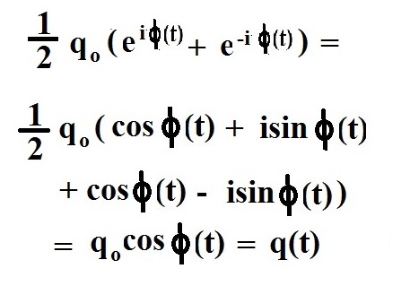
We can take q(t) and convert it into a wave-function expression:

As you can see, if we use Euler's identity and add the exponent to its complex conjugate, multiply by 1/2q, we get q(t). We now have a quantum expression we can use.

Since phi is time-dependent, and since the goal is to equate it with the relativity wave function, it is imperative that we make the relativity wave function time-dependent as well:

Note how position variables x, y, z were converted to time variables t1, t2, t3. We add these with t4 and multiply by coefficient a to get the observed time t. The four time dimensions may or may not add up to t which is why we multiply by a. We also multiply kct by A, B and C to make them equal to each expression in the phi function. We add those to get the final result: Dkct=phi(t). We use these equated expressions in the equated wave functions and their complex conjugates below:

Now we have the tools we need to calculate the gravitational waves' energy (E), the entropy (S), the temperature (T), the momentum (p), the velocity (c) and the acceleration due to gravity (g). Let's plug these wave functions into Schrodinger's time-dependant derivative expression and see what happens (but first we need to multiply both sides of the equation above by 2/q and subtract the complex conjugates):

Multiply both sides by a complex conjugate to get the expectation value:

At last! We get the energy (E). With a little algebra we can determine the entropy (S), the temperature (T), the momentum (p). We also get the velocity, which happens to be the speed of light (c). If we divide the velocity by t, we get an acceleration (g).

So there you have it!--a theory of quantum gravity based on something scientists claim they have observed and measured: gravitational waves.

Debunking D-branes and other Extra-dimension Myths

According to string theory, d-branes come in one or more dimensions. They provide an anchor for strings. Some string theories have only even-numbered d-branes; others have odd numbered d-branes. As we shall see later in this post, the odd d-branes, or systems with an odd number of space dimensions, have a better shot at being real. One real example is space in our universe. We perceive it as 3D, and it can be thought of as a giant 3-brane.

But what about 4-branes, 5-branes and beyond? Today we are going to put various multi-dimensional branes to a rigorous test. The test is designed to show whether extra dimensions truly exist. It is the cross-product test. The diagram below shows how the cross product works in three dimensions:

The results are in red. When we calculate the cross-product of two dimensions, we get a third dimension that is perpendicular to the others. To test for extra dimensions, we need to define what we mean when we say "dimension." Dimensions are lines in space that are perpendicular to each other.

Because they are perpendicular to each other, their cross-products must yield a kind of symmetry, i.e., there must be the same number of each dimension. The indexes can also be added or subtracted to get the cross-product. For example, in 3D space, D3D1 = D2 (3-1=2) and D1D2 = D3 (1+2=3) However, there must not be any index sharing. For example, D4D8 = D4 is invalid, since the D4 on the left side of the equation is clearly the same dimension as the D4 on the right. We could change the index(s) to cover our tracks, but then we lose the index symmetry--and such a loss reveals the problem in a different way.

We also need at least three dimensions to get started. Applying the test to 1-branes and 2-branes yields a bunch of zeros. But at least there is symmetry, so the dimensions in the 2-brane might be perpendicular. The fact there is no index sharing is also a good sign.

As you can see, I put the results in tables. Each row element and each column element yield a corresponding result in the tables (let your finger be your guide). Now let's look at a 3D system or 3-brane:

You'll notice cross-products that share the same index yield zero as they should. Three dimensions obey the index rule and have perfect symmetry. The bottom table above shows there are two results for each dimension. A 3-brane is perfect; it meets all the requirements, and we'll use it as a yard stick to judge systems and objects with extra dimensions.

Let's check out 4D:

The 4-brane isn't looking good. The results in red violate the index-sharing rule. There is also a lack of symmetry--there is not the same number of each dimension (see right-hand table). The cross-products are also fake. I'll explain what that means later when I'm done laying the groundwork. For now, let's move up to five dimensions:

Ah! Perfect symmetry! Four of each dimension. Could we be living in a 5D universe? A 5-brane sure looks feasible--but then there are those nasty index violations in red. Oh well.

The 5-brane does show, however, that odd numbers of dimensions have symmetry. What is true for five dimensions is also true for seven dimensions and the nine dimensions of E500 string theories:

Once again we have perfect symmetry and index violations in red. What about the 10 space dimensions of M-theory?

Holy d-brane, Batman! What a mess! Ten dimensions lack symmetry and have bleeding-red index violations. It's unlikely these dimensions are perpendicular to each other. But what about the 9D system? That one looks pretty good, not perfect like 3D, but close. Thus it is time to explain why its cross-products are fake as a presidential campaign promise.

If there are really nine dimensions of space then any cross-product between any two dimensions should yield the remaining seven--since the remaining seven are allegedly perpendicular to the two. The above tables only show single results for each cross-product. Such a strategy is useful in that it exposes which cross-products aren't perpendicular (see index violations marked in red). That being said, D1D2 should yield D9 and the rest. D3D6 should yield D8 and the rest. If these extra dimensions were real, there would be more uncertainty due to multiple results. We would not get a nice, single result from any cross-product. If we could choose the ideal d-brane or universe, 3D would be the best choice. The marvelous thing about 3D is you have perfect symmetry and the same number of dot-products as cross-products. With higher dimensions this is never the case.

The diagram above shows how D1D2 equals seven possible results in a 9D system. Such a system has 81 dot-products and 567 cross-products! Not exactly a balanced system. Then again, what if all those extra dimensions are tiny and curled up? That would sweep the multiple results under the rug. However, if dimensions are curled, their angles are no longer perpendicular. The diagram below shows the x-axis being curled to the y-axis. Note how the angle is no longer ninety degrees.

If dimensions don't have to be right angles to each other, then we can have an infinite number of them within right-angled 2D or 3D space.

The above diagram shows how a 2D triangle can be expanded into a 4D triangle that occupies a flat 2D space. But why stop at four dimensions when we can have eight or more?

As you can see, it is easy to fool ourselves into believing there are extra dimensions. What we call extra dimensions could really just be a bunch of posers occupying a flat 2D or 3D space. If there are really four or more dimensions that are right angles to each other, cross-product results would be uncertain. A lack of symmetry implies extra dimensions do not exist.

For more on this topic, check out theses links: "Debunking Bosonic String Theory's 26 Dimensions" and "Are String Theory's Extra Dimensions Real?" and How to Derive M-Theory's Eleven Dimensions and Reduce Them to Four Dimensions.

Why Are Quantum Energy Levels Discrete?

Why are quantum energy levels discrete in a potential well? What started out as a mathematical trick invented by Max Planck has become an established idea. Energies at the quantum level increase and decrease by integer multiples (n) of fh (frequency times Planck's constant). Let's plot a diagram to see what we can make of it.

The diagram above has a stair-step shape as energy levels go from n = 1 to n = 4. But what happens if we lay it on its side?

Now it looks like some sort of binary, oscillating wave. Let's smooth out the rough edges.

Yes, it most definitely looks like a wave. This is consistent with the fact that quanta are particle-waves. Since particles can behave like waves, it makes perfect sense that changes in energy would behave like waves as well. We measure the energy level when the wave peaks, and no energy is added or subtracted until the next peak.

Update: Below is a possible mathematical formula for the purpose of describing the wave-like character of changing energy levels.

It is the absolute value of a sine wave raised to the power of infinity. This causes all values to be zero or one. When the value is one, n increases or decreases by q; otherwise there is no change in n.

How to Derive M-Theory's Eleven Dimensions and Reduce Them to Four Dimensions

Today we are going to mathematically derive the eleven dimensions of M-theory. This is part three of a series of posts regarding the string theories. To fully understand what's going on here, I recommend you read "Debunking Bosonic String Theory's 26 Dimensions" and "Are String Theory's Extra Dimensions Real?"

Once again we have an x-y plane or system zooming along the z-axis with momentum p. The frequency of the ground-state oscillator is n/2. We want to add up all the values of n and get infinity minus one. At step one below we multiply the sum by the exponent e to the minus epsilon power--which is equivalent to multiplying by one. Epsilon is a very tiny number that is practically zero.

The sum is equivalent to minus one-half the derivative of the sum without multiplying by n.

Since the sum adds to infinity we can replace it with another expression that amounts to infinity: an exponent e divided by one minus the exponent e.

We then convert the expression's numerator and denominator into a Taylor expansion of exponent e, and then simplify.

Next, pull out one-over-epsilon from the fraction.

The variable s, like epsilon, is a tiny number. We can use the rule below to convert the denominator.

We can now multiply the numerator by the converted denominator. Note that the simplification leaves out the terms that cancel and have high powers of epsilon. These high-power terms drop to zero when epsilon goes to its zero limit.

We simplify further by multiplying the parenthetic terms by one-over-episilon, taking the derivative with respect to epsilon and multiplying by minus one-half.

We end up with infinity minus 1/8. We need a minus one, so we need to multiply -1/8 by eight. That gives us eight dimensions. Add to that the z-axis plus time--and we get a total of ten dimensions.

So then why does M-theory have eleven dimensions if there are only ten? Back in the 1990's there were five string theories. (Now there are around E500 string theories!) How could any of those theories be the unifying theory when there were five of them? M-theory to the rescue! According to M-theory, those five theories (or E500 theories) are just different forms of the same theory.

Imagine that each of the string theories describes a unique 10D universe. Imagine all those 10D universes existing in a higher dimension. Yes, the eleventh dimension. Think of the eleventh dimension as a line (or string if you prefer), and each 10D universe is a point along that line.

With a little math similar to what we were doing above, we can derive the eleventh dimension below. We take our infinity minus 1/8 (which includes the z-axis and time) and add up an infinite number of them.

We get infinity minus one. The minus one times one is one more dimension to add to our collection. That brings us up to 11D.

But as you probably know, we can also derive 26 dimensions. We can also derive four dimensions:

So how many dimensions does our universe have? Which mathematics is telling it like it is? Well, this is where our powers of observation come in handy. The most useful mathematical models are the ones that are consistent with the reality we observe. For now, it is prudent to go with 4D, since that is what we have observed.