Unifying the Dirac, Klein-Gordon and Einstein Equations

Within quantum field theory we find two equations based on Einstein's equation for energy (E = energy; p = momentum; c = light speed; m = mass):

The first is Dirac's equation. The second, the Klein Gordon equation (i = imaginary number; h-bar = Planck's constant; bold y with arrow = Dirac-Pauli matrices; a-sub-u = first derivative; psi = quantum field; t = time; up-side-down triangle = Laplacian).

The goal is to take elements and ideas from the above equations and combine them with Einstein's field equation below (Guv = Einstein's tensor; Gn = Newton's constant; Tuv = the energy-stress tensor; and then there's pi):

Let's first write Guv in quantum terms (psi-sub-r = relativity-field-wave function; Aj = a coefficient element in series j). Note there's a double derivative of psi with respect to an x-vector, and tensor indices (uv) after the closing parenthesis. There is also psi's complex conjugate, which, when multiplied my psi and the rest, gives the expectation value; i.e., a result we expect on the classical scale.

Next, we write Tuv in quantum terms (V = volume). Again we get an expectation value, and the entire term is placed in parenthesis and made a tensor with indices uv.

Now that we have Einstein's equation in quantum terms, let's define each element in greater detail. Below is the definition of psi:

If you are curious about the above arc-tangent term, click here. It has to do with quantizing spacetime.

Next we define k. The k represents wave number(s) for one or more particles summed (j=1 to n) by the summation sign. The arrow over k indicates it is a 4-vector. The "a" with a dagger is the creation operator. The zero in the ket represents the field in the ground state.

The variable x is also a 4-vector:

The bold b with an arrow can be any one of three types of spin matrices: Dirac-Pauli matrices (y) for half-spin particles; S-matrices for integer-spin particles; and the number one for zero-spin particles.

Below is a full demo of the Dirac-Pauli matrices:

Here is an example of one Dirac matrix acting on the k 4-vector:

The following are 4X4 matrices I designed for spin-1 particles. I always admired Dirac's equation and matrices, but they are limited to half-spin particles. Now it's possible to include bosons in the field.

We now have a quantized version of Einstein's field equations where we can work with both matter and anti-matter. We can work with zero-spin particles (Higgs field), spin-1 bosons, fermions, atoms, molecules and beyond ... and see how they curve spacetime in terms of the wave number(s) k.

The interesting thing about k^2 is it has the same units as Einstein's field equations: 1/L^2. Thus if we take the double derivative of psi with respect to x, we get k^2. Multiply that by the unit-less coefficient A; multiply psi by its complex conjugate--and we get the equivalent of an Einstein tensor element. Put 16 elements together and we get the complete Einstein tensor.

Unifying the Schwarzschild Metric and Quantum Physics

Is it possible to unify quantum physics with Schwarzschild's metric for black holes? Absolutely! All we need to do is adapt my relativity wave function to the task. For more information on the relativity wave function, click here.

Here is an example of the function:

It consists of Euler's identity and more than one k variable (bar-k's to be exact). Time is t; light speed is c, and i is an imaginary number. The variable rs below is the Schwarzschild radius; a and b are terms from the Schwarzschild metric, and r is the radius. Our first step is to transform the bar-k's. For example, bar-k(1) becomes ak(1).

Next, we trade Cartesian coordinates for spherical coordinates. Here is what we get:

We can now express the Schwarzschild metric in quantum mechanical terms:

When the partial derivatives above are solved, we get the standard Schwarzschild metric below:

Looks rather messy. Let's put the variables into a more manageable form:

When the function is used in Schrodinger's time-dependent equation (complete with potential energy V, the Laplacian, and Planck's constant, h-bar), here is what results:

Time to substitute the real values of a and b--but Huston we have a problem! Notice when r is equal to rs, we have zero on the equation's left side and infinity on the right side. The equation works fine as long as the particle is far far away from the black hole's horizon, i.e., when r is a big number. Under those circumstances, the equation reduces to a normal Schrodinger Hamiltonian.

It would also be nice if we had just one momentum term (p). So let's add up the squared momentums (p1, p2, p3). While we're at it, let's subtract the left side from the the right to get energy (E). When the particle is far from the black hole, E should be zero or close to it. As the particle gets closer to the black hole, E increases.

The Quantum Mechanics of Gravitional Waves

Today we are going to work out the quantum mechanics of gravitational waves using my relativity wave function. If you have no clue what I'm talking about, check out my post entitled "The New Relativity Particle Wave Function." The following video provides some basic information on g-waves:

Of course there are always naysayers. Here is a skeptic's video:

I didn't find the magnet demonstration very convincing. Magnets do a great job accelerating iron filings, but not wood chips. If the guy in the above video got those magnets to accelerate something non-metallic, I'd be impressed, but all he did was show magnetic field interactions under a bright light. Thus it seems like a safe bet to build a theory of quantum gravity based on the gravitational wave discoveries.

Below are some gravitational-wave equations we can work with. The first one is the chirp mass (Mc). It depends on two very big masses: m1 and m2. They could be a double-star system or a couple of black holes.

Next we have the scaling amplitude (q)--the size of the wave's stretching and squeezing (here is a link to an animation). Normally, the variable h is used, but later we are going to use h for Planck's constant along with h-bar. G is Newton's constant; c is light speed; distance is d; frequency is f, and there's pi.

Then there is the chirp (dot f). (For a demonstration of the chirp, see the video below .)

Next, we have the gravity-wave phase angle represented by the Greek letter phi. As you can see it depends on time (t). Below it is the chirp waveform amplitude q(t).

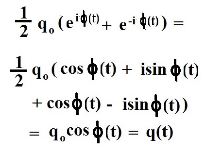
We can take q(t) and convert it into a wave-function expression:

As you can see, if we use Euler's identity and add the exponent to its complex conjugate, multiply by 1/2q, we get q(t). We now have a quantum expression we can use.

Since phi is time-dependent, and since the goal is to equate it with the relativity wave function, it is imperative that we make the relativity wave function time-dependent as well:

Note how position variables x, y, z were converted to time variables t1, t2, t3. We add these with t4 and multiply by coefficient a to get the observed time t. The four time dimensions may or may not add up to t which is why we multiply by a. We also multiply kct by A, B and C to make them equal to each expression in the phi function. We add those to get the final result: Dkct=phi(t). We use these equated expressions in the equated wave functions and their complex conjugates below:

Now we have the tools we need to calculate the gravitational waves' energy (E), the entropy (S), the temperature (T), the momentum (p), the velocity (c) and the acceleration due to gravity (g). Let's plug these wave functions into Schrodinger's time-dependant derivative expression and see what happens (but first we need to multiply both sides of the equation above by 2/q and subtract the complex conjugates):

Multiply both sides by a complex conjugate to get the expectation value:

At last! We get the energy (E). With a little algebra we can determine the entropy (S), the temperature (T), the momentum (p). We also get the velocity, which happens to be the speed of light (c). If we divide the velocity by t, we get an acceleration (g).

So there you have it!--a theory of quantum gravity based on something scientists claim they have observed and measured: gravitational waves.

Unifying Spacetime and the Forces

Let's start with a simple idea and expand on it. Imagine you have a total energy (E) and you subtract from that the energy of the strong, weak and electromagnetic forces. What do you have left? Gravitational energy.

Now we need something that represents the total energy. How about Schrodinger's Hamiltonian?

It's a good idea to express Schrodinger's Hamiltonian in terms of light speed squared (C^2). Why? Because light speed squared connects all the fundamental interactions (forces)--so we will set them all equal to C^2.

If we divide the Hamiltonian by mass (m) we set it equal to C^2. (C^2 = E/m.) Next, let's multiply each C^2 by time squared (t^2). Doing so gives us the spacetime metric. To make the terms equal, we should probably multiply each one by a coefficient K.

As you can see we've unified the forces and spacetime. What better way to spend a Sunday afternoon? The last equation, which is the spacetime metric, is just another way of saying, "Gravitational energy is equal to the total energy minus the other forces' energy."

In case you are curious, here are the variables: s is spacetime; z is the proton number; epsilon is the permittivity of free space; h-bar is Planck's constant; c is light speed; t is time; gij is the metric tensor. E is electricity; B is magnetism; I is current; p is charge density; Gn is Newton's constant; Gij is Einstein's tensor; Tij is the energy-stress tensor; Mh is the Higgs mass; g is the magnitude scaling constant; e is the natural exponent; m is the Yukawa particle mass; r is the particle radial distance; Fw is the weak force.

And let's not forget the equation for the Higgs field energy. The Greek letter there is the complex scalar field. H is its Hamiltonian (energy). The next term is kinetic energy and the last two terms are potential energy.

The New Relativity Particle Wave Function

General Relativity and quantum mechanics don't mix--so we are told by an echo chamber that has lasted a century. The Schrodinger time-dependent and time-independent equations don't fit with the 4D tensor format of Einstein's field equations. I decided to take on the challenge.

The root of the problem is the wave function (represented by the Greek letter psi). It depends on three space dimensions multiplied by a factor of k (momentum[p]/h-bar) and one time dimension multiplied by frequency (f).

To be compatible with relativity, we need to express the wave function in four spacial dimensions, where light speed times time (ct) makes up the fourth dimension. We multiply that by k4 to make it equivalent to frequency times time (ft).

Below are the mathematical steps needed to make an incompatible wave function into a compatible one. The variable A can be any coefficient for the exponent (exp()).

Notice the variable k has become four variables (k1, k2, k3, k4). The logic behind this will become clear when we test the new wave function later. For now, more variables offer more flexibility. They can all be equal to k or their values can vary depending on the situation.

We would very much like the the new wave function to do all the tricks the old one can do and then some. Let's do the time-dependent first-derivative test and see if the new wave function yields the same result as the old one. We set the variable A to 1.

Looks like a winner! Let's try the time-independent second-derivative test for the x-axis:

We do indeed get the same result for both wave functions. The only difference is the syntax. k becomes k1. Variable p^2 (momentum) becomes p1p1. It should be obvious that what works for the x-axis also works for y and z. So we can use this new wave function when working with Schrodinger's equation.

Now let's convert variables x, y, z, and ct to x1, x2, x3, x4. Let's see how well the new wave function works with a quantized version of the field equations. Uij is potential energy; h-bar is Planck's constant; m is mass; G is Newton's constant; c is light speed; V is volume; N is the large number of particles needed to make a little gravity; gijGij are scalar coefficients for each element of the rank-2 tensor created by the double partial derivative of the wave function psi along xi, xj.

With a little differential calculus and a pinch of algebra we can derive the field equations:

Notice how the wave function's complex conjugate is used to get the expectation value and eliminate the wave function psi.

Now I will show you the advantage of having more than one k variable. If we take double-partial derivatives of psi along k1, k2, k3 and k4, we can derive the spacetime metric and Lorentz factor. We can also derive yet again the field equations. You can see the details in my blog post entitled "Einstein's Field Equations Simplified."

OK, so we can derive a bunch of stuff with this new wave function. What's the big deal? Notice how we've unified General Relativity with quantum mechanics without invoking strings, branes or extra dimensions. Heck, we didn't even invoke the graviton. These things may or may not exist, but if they are never discovered we have a way to work with quantum gravity.

Since we don't need strings or extra dimensions to do this work, we have far less to prove than string theorists. We can make it work with established, empirically verified physics--and they can't. That puts us way ahead of the curve.

Derive the Field Equations From the Uncertainty Principle

Heisenberg's Uncertainty Principle is General Relativity in disguise. Let me show you. Begin with the Uncertainty Principle. The variables are momentum (p), position (x), Planck's constant (h-bar).  Work through equations 1 through 3 below to get 4.  Notice how an increase in p causes a decrease in x and vice versa.  Somehow this seems eerily familiar.

At 5 and 6 below, we do a dimensional analysis and see the terms are all numbers divided by a line squared (L^-2). The field equations are formatted this way. Notice the "curved space" is an increase in the change in momentum (p) and a decrease in the change in space (x). The new variables are Newton's constant (G or Gn), volume (V), light speed (c), energy (E).

With equations 7-9 we derive Einstein's field equations featuring Einstein's tensor (Gij) and the energy-stress tensor (Tij). Oh ... and let's not forget 8pi.

Now let's derive the other Uncertainty Principle ... you know ... the one with energy and time?

Now, just for fun, let's go back to equation 5 and, from there, derive a quasi-Schrodinger/Einstein equation, which features the Hamiltonian energy (H) the Greek letter psi, the metric tensor (gij), and N for a large number of particles. To get a little gravity, you need a huge number (N).