How to Derive the Laplace Operator "Laplacian" for Spherical, Cylindrical, and Cartesian Coordinates

If you study physics, time and time again you will encounter various coordinate systems including Cartesian, cylindrical and spherical systems. You will also encounter the gradients and Laplacians or Laplace operators for these coordinate systems. Below is a diagram for a spherical coordinate system:

Next we have a diagram for cylindrical coordinates:

And let's not forget good old classical Cartesian coordinates:

These diagrams shall serve as references while we derive their Laplace operators. Here's what they look like:

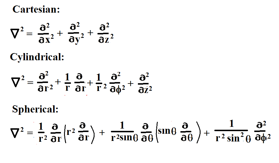
The Cartesian Laplacian looks pretty straight forward. There's three independent variables, x, y, and z. The operator has three terms as one would expect, but check out the cylindrical operator--it has four terms and three variables. What's up with that? If you examine both the cylindrical and spherical operators, you notice terms that have factors in front of the partial derivative operators. Where do they come from and why are they necessary? To answer such questions, it pays to derive these operators from scratch.

In this post, we derive all three Laplace operators, so a side-by-side comparison can be made which further illuminates the logic behind the derivation procedure. Let's begin by expressing an arbitrary vector S in terms of each coordinate system:

The next step is to extract the unit vectors. This is done by taking partial derivatives of S with respect to each variable. For the Cartesian version, this is totally straight forward:

No normalization is required because dot products of the unit vectors give you 1's and 0's as expected:

Now, here's what we get when we take partial derivatives of the cylindrical version of S:

The unit vectors we get aren't really unit vectors. When we do dot products, we don't necessarily get 1's and 0's. Normalization is required:

Notice that one of the partial-derivative operators requires a normalization factor of 1/r. Spherical unit vectors also require normalization:

Here, two spherical partial-derivative operators require a normalization factor: 1/r and 1/rsin(theta) respectively. Now that we know the normalization factors, we can construct the gradients:

Notice how the unit vectors are placed in front of the partial-derivative operators. A common mistake is to place the unit vectors after the operators like this:

This is technically wrong or should be, since the operators are acting on the unit vectors! Here's what happens:

So we keep the unit vectors in front. This prevents errors and frustration as we perform the next step which is to square the gradients to get the Laplace operators. Let's do the easiest one first, the Cartesian gradient. We multiply each term by every other term. Doing so allows us to construct this matrix:

Here's a couple of examples of the multiplication procedure. Note that the product rule of derivatives is employed and the partial-derivative operators do in fact operate on the unit vectors, but only where it's appropriate:

The final answer is ...(drum roll) ...

Now let's square the cylindrical gradient using a similar procedure:

Looking at each term it is obvious, that once again, there is a partial-derivative operator acting on a unit vector. We can make a list of each operation we will encounter, then use the list data to make the necessary substitutions during the multiplication process.

And here's the math for the cylindrical Laplacian:

Here's the final answer:

Finally, we tackle the spherical Laplacian:

The second matrix above indicates which terms give us zero when we do the math. Below we focus on the terms that yield a value other than zero:

We gather up the terms:

Too many terms! Here's what we can do. Let's take the first couple of terms and factor out 1/r^2. Then apply the derivative product rule in reverse:

Next, take the following terms and factor out 1/{(r^2)sin(theta)}. Once again, apply the product rule in reverse:

After making substitutions, the final answer is ... (fireworks) ...

How to Create Your Own Famous Physics Equation

So you've learned a bunch of physics equations that describe a whole bunch of phenomena. The most famous, of course, is E=mc^2. But maybe you have made some observations and have collected some data that no famous equation can model effectively. So what do you do now? Well, it's time for you to make your mark in this physics world! It's time to learn how to create your own physics equations.

Many things in nature can be modeled using differential equations or equations with a polynomial and/or multinomial pattern. For example, the ionization energies of electrons follow a polynomial pattern (click here to learn more).

Your mission, if you choose to except it, is to find the function, f(x), that fits your data set. To help you get started, let's review the concept of the slope or derivative. We know the derivative of f(x) is as follows:

Normally the value of h is a small number with a zero limit. But we're going to set h to 1. Here's what we get:

Because we set h to 1, equation 5 shows we can determine the slope with just the numerator of equation 1. Below we list the f(x) data. We then take each f(x) value and place it in a line. The next step is to subtract adjacent values, then take the results and repeat the process until we get zero. It makes a nice up-side-down triangle:

Notice what we did above. The process is equivalent to taking successive derivatives of f(x). We end up with zero, but before that we have a constant equal to 4. To get 4, we performed the equivalent of a double derivative. So to find f(x) it makes sense to backpedal, i.e, find the double integral of 4:

Now we're getting somewhere. We just have to find the values of b and c. Looking at the data, it is apparent that when x is 0. f(x) is 1. Thus, the constant c equals 1:

We find the value of b as follows:

So b is zero. When we put it all together we get our final equation:

Now, the above method works fine if you have one input variable and one output of f(x), but what if there's two or more input variables? Suppose you are trying to find the equation for f(x1,x2,...xn)? Let's try the following:

We can see right away that when x and y are set to zero, we get a constant of 5:

The trick to finding a multi-variable function is setting all input variables to zero except for the one you are working on. Also, to make life simpler, subtract the constant. Let's work with variable x:

Our up-side-down number triangle gives us a constant of 12. Now let's do the integral, but before we do, notice there's three steps to getting the constant. That's the equivalent of a triple derivative, so we need a triple integral:

Next, we solve for coefficient "a":

Then there's coefficient "b":

Our polynomial for x is as follows:

Now let's find the polynomial for y using the same methods we used for x:

Add the y-polynomial to the x-polynomial and add the constant 5 (which nets -5). We are finished if x and y are orthogonal, since any mixed terms would just be zero. But what if mixed terms may exist? To determine if they do or don't, let's label the current function g(x,y).

Subtract g(x,y) from f(x,y). The result, h(x,y), should equal zero if x and y are orthogonal. If h(x,y) doesn't equal zero, there's mixed terms we need to find.

After doing the subtraction, we see that no h(x,y) value is zero.

Using equation 21 and the h(x,y) results, we can build a system of linear equations and solve for A, B, and C:

To find B, double equation 22 and subtract it from 23. To find C, plug in the value for B at equations 23 and 24, then double equation 23, subtract 24. To find A, plug in the the values for B and C into equation 22.

Finally, plug in the values for A, B, and C at equation 21, then add that to g(x,y) to get f(x,y):

You now have the equation that will make you famous! Well, not really, but you have a systematic methodology that enables you to find a function that fits the data.

Update: There are data sets where many of the input variables are unknown or not precisely known. Some examples include weather, turbulence, climate, the stock market, etc. Finding a function seems impossible, but such a function can be converted to a time-series function, where the only input variable is time. At each given time you have g(t)+ epsilon(t) which is equal to f(a1,a2...an).

The blue dots in the above chart represent the scatter-plot data. The black line represents the average or g(t) for each t. At 27 through 30 below the variance (epsilon(t)) is determined for each value of t:

The chart can be split up into sections (q,r,s,u,v). Each section has an exponential or logarithmic curve, or a straight line. Straight lines can be modeled using a linear equation with a slope and intercept (see 31 below). The math is simple. To model the curves, convert the data into straight lines, find the linear equation, then take the log or exponential of that equation. The table below details the process and also shows how to handle horizontal and vertical lines:

The final step is to create a system of equations for g(t):