How to Create Your Own Famous Physics Equation

So you've learned a bunch of physics equations that describe a whole bunch of phenomena. The most famous, of course, is E=mc^2. But maybe you have made some observations and have collected some data that no famous equation can model effectively. So what do you do now? Well, it's time for you to make your mark in this physics world! It's time to learn how to create your own physics equations.

Many things in nature can be modeled using differential equations or equations with a polynomial and/or multinomial pattern. For example, the ionization energies of electrons follow a polynomial pattern (click here to learn more).

Your mission, if you choose to except it, is to find the function, f(x), that fits your data set. To help you get started, let's review the concept of the slope or derivative. We know the derivative of f(x) is as follows:

Normally the value of h is a small number with a zero limit. But we're going to set h to 1. Here's what we get:

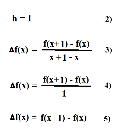
Because we set h to 1, equation 5 shows we can determine the slope with just the numerator of equation 1. Below we list the f(x) data. We then take each f(x) value and place it in a line. The next step is to subtract adjacent values, then take the results and repeat the process until we get zero. It makes a nice up-side-down triangle:

Notice what we did above. The process is equivalent to taking successive derivatives of f(x). We end up with zero, but before that we have a constant equal to 4. To get 4, we performed the equivalent of a double derivative. So to find f(x) it makes sense to backpedal, i.e, find the double integral of 4:

Now we're getting somewhere. We just have to find the values of b and c. Looking at the data, it is apparent that when x is 0. f(x) is 1. Thus, the constant c equals 1:

We find the value of b as follows:

So b is zero. When we put it all together we get our final equation:

Now, the above method works fine if you have one input variable and one output of f(x), but what if there's two or more input variables? Suppose you are trying to find the equation for f(x1,x2,...xn)? Let's try the following:

We can see right away that when x and y are set to zero, we get a constant of 5:

The trick to finding a multi-variable function is setting all input variables to zero except for the one you are working on. Also, to make life simpler, subtract the constant. Let's work with variable x:

Our up-side-down number triangle gives us a constant of 12. Now let's do the integral, but before we do, notice there's three steps to getting the constant. That's the equivalent of a triple derivative, so we need a triple integral:

Next, we solve for coefficient "a":

Then there's coefficient "b":

Our polynomial for x is as follows:

Now let's find the polynomial for y using the same methods we used for x:

Add the y-polynomial to the x-polynomial and add the constant 5 (which nets -5). We are finished if x and y are orthogonal, since any mixed terms would just be zero. But what if mixed terms may exist? To determine if they do or don't, let's label the current function g(x,y).

Subtract g(x,y) from f(x,y). The result, h(x,y), should equal zero if x and y are orthogonal. If h(x,y) doesn't equal zero, there's mixed terms we need to find.

After doing the subtraction, we see that no h(x,y) value is zero.

Using equation 21 and the h(x,y) results, we can build a system of linear equations and solve for A, B, and C:

To find B, double equation 22 and subtract it from 23. To find C, plug in the value for B at equations 23 and 24, then double equation 23, subtract 24. To find A, plug in the the values for B and C into equation 22.

Finally, plug in the values for A, B, and C at equation 21, then add that to g(x,y) to get f(x,y):

You now have the equation that will make you famous! Well, not really, but you have a systematic methodology that enables you to find a function that fits the data.

Update: There are data sets where many of the input variables are unknown or not precisely known. Some examples include weather, turbulence, climate, the stock market, etc. Finding a function seems impossible, but such a function can be converted to a time-series function, where the only input variable is time. At each given time you have g(t)+ epsilon(t) which is equal to f(a1,a2...an).

The blue dots in the above chart represent the scatter-plot data. The black line represents the average or g(t) for each t. At 27 through 30 below the variance (epsilon(t)) is determined for each value of t:

The chart can be split up into sections (q,r,s,u,v). Each section has an exponential or logarithmic curve, or a straight line. Straight lines can be modeled using a linear equation with a slope and intercept (see 31 below). The math is simple. To model the curves, convert the data into straight lines, find the linear equation, then take the log or exponential of that equation. The table below details the process and also shows how to handle horizontal and vertical lines:

The final step is to create a system of equations for g(t):

A Perturbation Theory Proof

To prove the validity of the perturbation expansion, let's start with a simple and obvious statement:

It seems intuitive that a variable x can be the sum of two terms containing two new variables. In fact, the same can be said of variable a1:

And, a2 can be the sum of two terms containing two new variables. We can repeat this exercise as many times as we like until we reach a(sub-n):

Using equations 2 through 5 we make a series of substitutions which transform equation 1 into the familiar perturbation expansion:

However, equation 6 is an exact solution which can't be had unless we know the value of a(sub-n). Let's assume we don't. Let's eliminate a(sub-n). If we do, we get an approximate solution:

Now, how do we apply this approximate series known as a perturbation series? Consider a function of x:

Let's assume this function of x is too hard to solve. So we re-write f(x) above to show the easy, solvable part and the seemingly unsolvable part:

Let's suppose the hard part is g(x). Wouldn't it be great if we could just get rid of it? Not permanently. Just for the time being. We do away with g(x) by multiplying it by epsilon, and epsilon has a zero limit.

We end up with equation 12 which is easy to solve. The solution can be found at 13. However, we didn't solve variable x--we solved what is called an unperturbed x or x0. We can now plug that solution into equation 7 and equation 8. Because x is approximately equal to x0 plus the rest of the series, we can make a substitution at equation 11 to get the following:

At 15 we set the equation to zero. The idea here is to solve the xi coefficients. This is often done by grouping terms on the basis of their epsilon powers. The equation is broken up into smaller, simpler equations that are easy to solve. At 18 below, the solved coefficients are plugged into the series and epsilon is set back to 1 (giving us back the equivalent to the missing hard part of the original equation). At 19 and 20 we simply add up the coefficients to get a close approximation of the true value of x.

Since the intent of this post was to do a general proof of perturbation theory, no specific problem-solving examples were provided. Click here to see an example of a specific problem solved using perturbation theory.

How to Falsify the Holographic Principle

Does the surface of a black hole contain its information? Is our universe really a hologram? In the video above, Leonard Susskind makes the case, but Karl Popper would no doubt scream, "Where's the evidence!" So to keep Karl Popper from rolling over in his grave, we will attempt to falsify the holographic principle.

According to the holographic principle, the maximum amount of information in a region of space is proportional to the area of the region--not the volume! That seems counter-intuitive. It's as if a black hole's surface area, for instance, is like a holographic plate storing all the black hole's information. The black hole entropy equation is based on this assumption or vice versa:

However, we could make up a new principle that states the following: The maximum amount of information in a region of space is proportional to the area of Cleveland Ohio. We could postulate that all information from each black hole ends up in Cleveland. Here's the equation:

Granted, using the area of the black hole seems more convenient, but as we shall demonstrate, the area used in the equation is arbitrary. Let's assume for five milliseconds that the black hole's surface area is not really a holographic plate. Why is the information proportionate to area rather than volume? To answer this question we need to review some basic laws of motion. Consider an acceleration vector. It has units of distance per time squared:

Now, take note that the distance D is not any particular distance; it's just a unit or dimension. In fact it's one dimension, not two, not three. OK, suppose there's a particle accelerating along one dimension of space. It propagates a distance of x. That gives us the following:

On the right side of equation 4 above, we have x times D--that makes an area:

What exactly is this area A? Is it the area of a black hole or Cleveland? It's not the area of anything, but if we want, we can pretend it is the area of a black hole. The choice is completely arbitrary. Now let's take this non-existent area A and place it into an entropy equation:

The area in equation six is not any particular area, including a black hole's. However, equation six could be used to model the entropy of a black hole notwithstanding. So it's true that a black hole's entropy or information is proportionate to an area, but it is also proportionate to a volume:

Using a little algebra we derive 11 below:

Looking at 11 we can infer that the maximum amount of information in a region of space is proportional to area or volume. However, to calculate the information using the volume requires we know the pressure (or energy density) and the black hole's temperature as well as the volume. If we know the area, then we know all we need to know to calculate the information. Therefore, a principle involving the area instead of the volume is more convenient--and most likely has nothing to do with holograms.

An Analysis of Alcubierre's Warp Drive

"By a purely local expansion of spacetime behind the spaceship and an opposite contraction in front of it, motion faster than the speed of light as seen by observers outside the disturbed region is possible."--Miguel Alcubierre

To read Alcubierre's original warp drive paper, click here. First, let's derive Alcubierre's warp-drive metric from Einstein's field equations. Here is a list of variables required:

We begin with equation 1, Einstein's famous general relativity equation, then we do a little algebra and contract the tensors to simplify the math:

Next, we put together the metric. Equation 12 below is the finished product:

Coordinates y and z are set to zero because the spaceship is moving along the x axis. Velocity v is further defined below. It is a function of the warp-bubble shaping function and the difference between the spaceship's position and the total distance along x.

At 15 notice the value inside the warp bubble is 1 and outside is zero. This allows time to dilate outside the warp bubble, while inside the bubble there is no time dilation. More on this later. For now, let's continue defining the other components:

Below is a crude diagram representing the warp bubble moving along the x axis:

"It is then easy to see that for the spaceship’s trajectory we will have: dτ = dt ."--Miguel Alcubierre

From Alcubierre's metric we can derive a Lorentz equation (see 19 below) that shows how time dilation is avoided. Since the value of the bubble shaping function is 1 inside the warp bubble the velocity v and velocity x/t cancel each other, so there's no time dilation inside the warp bubble. The function value is 0 on the outside, so there x/t is not cancelled and any time dilation would take place outside the warp bubble.

At 20 above, we see that proper time (t') equals coordinate time (t).

"The metric I have just described has one important drawback, however: it violates all three energy conditions (weak, dominant and strong). Both the weak and the dominant energy conditions require the energy density to be positive for all observers."--Miguel Alcubierre

It appears that negative energy density is required to achieve speeds greater than light speed. Negative energy density implies negative energy and negative mass. Check out the following equation system:

Notice that when v > c, the only way to get a value for m' that is real and not imaginary is to plug in -mv^2, a negative energy that has negative mass (-m). For photons, where v = c, mass m' is zero as expected. Particles that move faster than light (e.g. tachyons) have negative mass. Thus it seems such exotic matter is required to achieve superluminal speed. However, consider a satellite orbiting a black hole at radius r:

The black hole has positive mass, i.e., positive energy density. If we increase that positive energy density, we can imagine the satellite orbiting faster and faster. There seems to be no upper limit to velocity v in this gadanke experiment, since there is no apparent upper limit to positive mass m. Further, using Einstein's field equations we can show that unlimited positive energy density (pressure, heat, etc.) can yield unlimited velocity:

At equation 30 above it is plain to see that any increase in positive energy density on the right side will cause a corresponding increase in velocity on the left side. So it appears exotic matter is not really needed to achieve superluminal speed. But then there's this:

"[L]ight itself is also being pushed by the distortion of spacetime."--Miguel Alcubierre

This is an unfortunate choice of words. It gives the impression that the distortion of spacetime can push light faster than light. At least that's what needs to happen if the spaceship is going faster than light; otherwise, the ship's electromagnetic energy could be left behind! Let's see what happens to photons when spacetime is distorted:

On the left side of equation 36 we have a mass particle with velocity v. On the right we have a photon with frequency f. If velocity v increases due to spacetime distortion, the velocity of the photon does not increase; rather, its frequency increases. Now, just for fun, what would happen if we assume the photon's velocity could increase?

On the right side of equation 38, the denominator has c'--a special photon velocity that can rise above c. What is the consequence? A paradox! When energy density increases, so does the spacetime curvature on the left side. This causes c' to increase wich causes the spacetime curvature to reduce which causes c' to reduce and so on. Bottom line: you end up with some very screwed-up physics!

If we can't show that photons go faster than c, at least we can show that other particles can ... or can we? Imagine the spaceship moving toward a star system at velocity nc, which is greater than c. The star system sends photons toward the spaceship at velocity c. What is the combined velocity? It's not nc + c. The velocity addition formula reveals the answer:

As Einstein himself could have told you, the combined velocity is no faster than light! This means no matter how fast distorted spacetime moves the spaceship, if there are any photons along its path (and there will be!), it will move no faster than light.

So how should we interpret equations 30 and 33? Why does it appear that superluminal speed is possible? Equation 33 makes sense if we place ourselves inside the spaceship and allow time dilation to happen.

At 43 above, we multiply the real velocity by t to get the distance. The perceived velocity v is that distance over proper time t', the time experienced by the observers in the spaceship. Let's see what we can derive:

At 51 above, we see that as epsilon gets closer to 1, the perceived velocity gets closer to infinity. The real velocity (epsilon-c) never goes faster than light.

We can determine the value of alpha for equations 30 and 33 (see equation 55):

Now equations 30, 33 and 52 make sense when you consider that observers outside the spaceship will see it going no faster than c, but observers inside the spaceship will swear they covered distance vt in time t', which could be faster than light.

But then again, we have a time dilation problem, since the clock inside the spaceship won't agree with the clock of outside observers. This is definitely true if the spaceship moves and its departure point A and arrival point B are at rest. We illustrate this in the diagram below. The arrow represents the spaceship.

But what if the spaceship, points A and B move at the same rate?

If points A, B and the spaceship all move at the same rate as in the above diagram, their clocks will agree. All observers along that path will be under the impression that the spaceship traveled distance vt in time t', which could be faster than light, at least on paper.

Now, if the observers in the spaceship view the star system they're heading for, according to the velocity addition formula, the combined velocity of the ship and the photons coming from the star will not exceed light speed, so what do they see? We can speculate they see a shorter distance or distance vt' instead of distance vt. If they don't look where they are going, they might assume the distance is vt and conclude they covered it faster than light.

Given what we now know, we should be able to visit any star system in record time, and when we get back home, our clock will agree with clocks on earth. Albeit, Miguel Alcubierre's paper makes no mention of the impact the needed energy will have on the spaceship's clocks. Things like mass and energy also slow time. According to Varieshi and Burstein's paper (click here to read), the amount of energy (mass) needed to manipulate spacetime to achieve a seemingly superluminal speed is approximately 3.42 X 10^38 solar masses! Many orders of magnitude greater than our observable universe! So time dilation is a problem even if we can successfully get the spaceship and points A and B moving at the same rate.

Conclusion: Warp drive makes wonderful science fiction--and it will be quite some time before it becomes a scientific fact.

Update: So do we really need the spaceship and points A and B moving at the same rate to cure time dilation? Take the muon time dilation experiment. When muons are moving at velocity v, their time slows. But if an observer were riding the back of a muon and considered herself at rest, she would see the scientists moving at velocity v, so why doesn't their time dilate as well? If the muons and scientists that observe them are moving at v relative to each other, shouldn't their clocks agree?

But then a closer look at the Lorentz factor reveals what's going on. Time dilation really depends on how fast the muons and scientists are moving relative to the speed of light--and not to each other. Thus the scientists really are at rest (or slower than the muons)--a photon has no trouble catching them, but does have trouble catching a fast muon (according to a coordinate-time observer; a proper-time observer [the muon or scientist] will see the photon approaching at c). Thus, for their clocks to agree, points A, B and the spaceship must move at the same velocity relative to the speed of light, not to each other.